 Let’s say you have shipped 1,000 products to your customer on January 1st. All are immediately placed into service. And each month since you have received a few product returns, what we are going to call failures. We also have fitted the data to a Weibull distribution. Then in May, your boss asks you to estimate how many failures to expect in June.
This is a simple example as we’re not shipping units every month, nor changing the product design or assembly process. We also have worked out the fitted Weibull parameters already. That leaves the calculation of how many failures we should expect over the next month.
The Problem and Assumptions
We want to know how many product returns will arrive next month. We have a pattern of observed product returns over the past 5 months. Thus our first assumption is the pattern will continue. Of course, it might not.
The statistics won’t help us justify this assumption, we would need detailed failure analysis of all failures plus an understanding of different types of actual and potential failure mechanisms. If something starts or stops failing over the next month at a different observable rate then our estimate will be wrong. We have the potential to be surprised.
Given the data and no other information, we assume the pattern will continue and we can base our estimate on the data available.
Of course, there are many other assumptions. That all customers report failures accurately and in a timely manner. That all units that started operation have not been retired or replaced without being reported to us. That the products were not modified by the customers. That all the customers use the products in a similar manner and in similar environments. The fitted parameters represent the data and population behavior well.
We make assumptions to allow a calculation, yet understanding the assumptions allows us to gather the important information that improves our ability to estimate the expected number of returns. It does complicate our calculations and does improve the estimate, yet has a cost of the need for more data and better models.
The Approach
There is more than one way to estimate the number of failures next month, yet I find using the Weibull cumulative density function (CDF) is straightforward. The CDF provides the probability of failure over a duration, t, starting from time zero.
So, if we calculate the probability of failure, times the number of units that have the potential to fail (units shipped in this example) we have an estimate of how many should fail over that duration.
The fitted data and the CDF formula times the 1,000 units should provide a number of failures over the first 5 months that is similar or close to the number of failures actually received. The data we have received was the basis for the fitted parameters, and we would expect the calculated result to be close to the actual result.
Then let’s calculate the probability of failure from time zero to the end of 6 months, the end of the coming month. Times the number of units shipped, and minus the number expected to fail over the first 5 months results in how many to expect next month.
Some Calculations and Answer
Let’s say we have witnessed 28 failures over the first 5 months (150 days or 3,600 hours) and have fitted a Weibull distribution based on the time to failure (the difference between January 1st, or the date of shipment, and when the failed units returned). We probably should use days as the unit of measure since we do not have data supporting anything more precise.
Our fitted Weibull parameters are Beta of 0.78 and Eta of 14,583 days. The Weibull CDF formula is
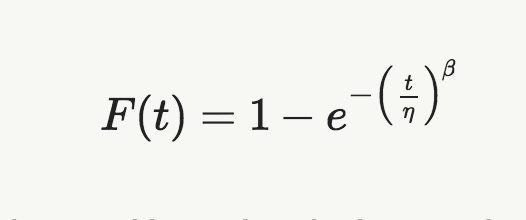
Setting time, t, to 150 days and inserting the beta and eta values, we calculate the probability of failure as 0.02776. This probability times the 1,000 units estimate the number of failures over 150 days as 27.76, which rounds off to 28, the number we observed.
Now set time, t, to 180 days, or the end of the next month. Run the calculation we get 0.03194. Times the 1,000 units and we would expect 31.94 or 32 failures over the 6 months.
To estimate how many new failures will arrive in June, subtract the number of failures over the first 5 months from the number expected over 6 months, 32 – 28 = 4. Therefore, we can report to our boss we expect 4 failures in June if all the assumptions are true enough.
Summary
The math is pretty easy. Understanding and checking assumptions is the key. If any of our assumptions are significantly wrong our estimate will be wrong. To get a good estimate you need good enough data. Often our work is finding the balance between what data we have and how well that will represent the reality which we are trying to estimate or model.
Using the fitted distributions data provides a way to estimate the failures to expect in the next month, quarter or year. The further out in time you forecast the more risk that one or more assumptions will not be true enough. It’s a risk we take.
Bio:
Fred Schenkelberg is an experienced reliability engineering and management consultant with his firm FMS Reliability. His passion is working with teams to create cost-effective reliability programs that solve problems, create durable and reliable products, increase customer satisfaction, and reduce warranty costs. If you enjoyed this articles consider subscribing to the ongoing series at Accendo Reliability.